TL;DR: Modern LLM training is long and costly. To plan the best configuration of compute, model size \(N\), and dataset size \(D\) for a test-loss target, scaling laws are fit by training small models and modeling the relationship between compute, \(N\), \(D\), and test loss. That relationship is then extrapolated to bigger models.
This is my summary of Scaling Laws, Carefully
Rosenfeld Et Al Scaling Laws (2020)
Modeling the error as a joint function of both model size and data size, across a diverse set of architectures (ResNet, WRN, LSTM, Transformer) and optimizers (Adam, SGD variants). They developed an empirical ML loss prediction model and observed that, holding one axis fixed, the error decays as a power law in the other:
$$ \hat{L}(D, N) \approx \frac{A}{N^{\alpha}} + \frac{B}{D^{\beta}} + E $$where \(D\) is the dataset size, \(N\) is the model size, and \(E\) is the irreducible loss, the part that does not depend on \(N\) or \(D\). \(A\), \(B\), \(\alpha\), and \(\beta\) are the optimized parameters.
In the settings examined by Hestness et al., model improvements shifted error without noticeably changing the observed power-law exponent.
Kaplan Et al.’s Scaling Laws (2020)
This work brought the laws to Transformer language models, with experiments from 768M to 1.5B non-embedding parameters and 22M to 23B tokens. Its findings aligned with previous work.
Their derived scaling law was
$$ \hat{L}(N,D) = \left[ \left(\frac{N_c}{N}\right)^{\frac{\alpha_N}{\alpha_D}} + \frac{D_c}{D} \right]^{\alpha_D} $$Some insights of this work:
- Larger models reach a given loss with fewer optimization steps and fewer data points than small models (sample efficient).
- The data needs to grow in a specific proportion to the growth of the model size to avoid training being data-limited. \(N^{\alpha / \beta} / D\).
- Given a fixed compute budget, it is more efficient to train a very large model and stop before convergence than to train a smaller model all the way to convergence. This finding is where the Chinchilla scaling laws (the next section) disagree.
Chinchilla Scaling Laws (2022)
This work tackled the question of what is the best strategy for allocating resources given limited FLOPs
$$ N_\text{opt}(C), D_\text{opt}(C) = \operatorname*{arg\,min}_{\text{s.t. } \text{FLOPs}(N,D) = C} \hat{L}(N, D) $$The authors reached similar optimal parameters with three different methods. This showed that the previous power laws created under-trained models, and that the dataset should be scaled roughly equally with the model size:
- Instead of “grow the model faster than the data” (\(N_\text{opt} \propto C^{0.73}\)), for every doubling of model size, you should also double the number of training tokens (\(N_\text{opt} \propto C^{0.5}\) and \(D_\text{opt} \propto C^{0.5}\)).
- Instead of “train a big model and stop before convergence,” you should train a smaller model on more data.
Under the same compute budget as Gopher (Rae et al. 2021; 280B parameters, 300B tokens), Hoffmann et al. trained Chinchilla (70B parameters, 1.4T tokens), and it outperformed Gopher across the board.
Scaling Laws in Data-Limited Region
One of the hypothesized limitations of modern LLMs is not having enough data (hitting a data wall). The above power laws were derived assuming \(D\) contains high-quality, cleaned, unique data.
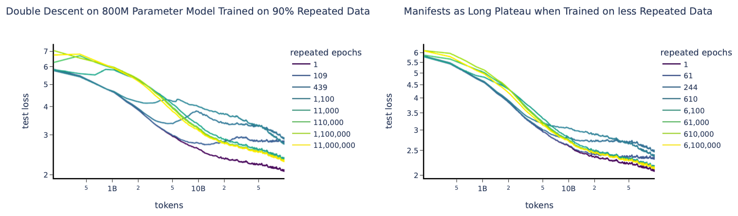
In the finite-data regime, Hernandez et al. (2022) observed the double-descent phenomenon: they took a dataset and changed the ratio of duplication it contains. The test loss gets worse and then better again as a function of how much the repeated data is emphasized.
Muennighoff et al. (2023) then updated one of the Chinchilla parametric fits to use effective (discounted) data and model size in place of the raw quantities:
$$ \hat{L}(N, D) = \frac{A}{N'^\alpha} + \frac{B}{D'^\beta} + E $$where the discounted counts are
$$ \begin{aligned} D' &= U_D + U_D\, r_D\left(1 - \exp\!\left(-\frac{R_D}{r_D}\right)\right) \\ N' &= U_N + U_N\, r_N\left(1 - \exp\!\left(-\frac{R_N}{r_N}\right)\right) \end{aligned} $$\(U_D\) is the number of unique tokens, \(R_D\) is the number of repeats, and \(r_D\) is a learned half-life. \(U_N\), \(R_N\), and \(r_N\) are the same three quantities for model size.
- The intuition is that a token’s value decays exponentially as it is repeated.
- Larger models overfit more quickly on repeated data.
References
- Deep Learning Scaling is Predictable, Empirically, Hestness et al., 2017.
- A Constructive Prediction of the Generalization Error Across Scales, Rosenfeld et al., ICLR 2020.
- Scaling Laws for Neural Language Models, Kaplan et al., 2020.
- Training Compute-Optimal Large Language Models, Hoffmann et al., NeurIPS 2022 (Chinchilla).
- Scaling Language Models: Methods, Analysis & Insights from Training Gopher, Rae et al., 2021.
- Scaling Laws and Interpretability of Learning from Repeated Data, Hernandez et al., 2022.
- Scaling Data-Constrained Language Models, Muennighoff et al., NeurIPS 2023.
- Scaling Laws, Carefully, Lilian Weng, Lil’Log, 2026.