Causal inference is essential for informed decision-making, as it uncovers the true data-generating processes beyond mere associations found in predictive models. The fundamental challenge in causal effect estimation is that we see the outcome under the treatment a sample received. We do not see the outcome that sample would have had under the other treatment.
Short recap from \[1/2\] Estimating a Treatment Effect with Causal Inference:
- Conditional average treatment effect (CATE) \(\tau(x) = \mathbb{E}[Y(1) - Y(0) \mid x]\). The effect of treatment for a sample with features \(x\).
- ATE \(\mathbb{E}[\tau(x)]\). The average of the CATE over samples. A randomized difference of means.
- Outcome model \(\mu(x, t) = \mathbb{E}[Y \mid x, T=t]\). A supervised model of the outcome.
Inverse Probability Weighting for Average Treatment Effect Computation
For a randomized controlled experiment there is a simple estimator of the ATE:
$$ \operatorname{avg}(Y \mid T=1) - \operatorname{avg}(Y \mid T=0). $$However, a randomized controlled experiment is often not feasible. We therefore aim to turn an observational study into something that looks like a randomized controlled experiment. In an observational study, there is a bias in which samples take which treatment:
$$ p(x \mid T=0) \neq p(x \mid T=1). $$The inverse propensity weight reweights the samples so they have the same weighted distribution. We can then use that weight to simulate a randomized experiment, with the following procedure:
- Use any ML method to estimate
- Compute the average treatment effect with
Downsides of this weighting:
- Calibration is important since we use the probability value.
- We need to estimate the propensity score, which is a difficult ML task.
- If there is not much overlap between the treatment groups, the propensity scores are easily miscalibrated.
- Weighting by the inverse can create large variance and large errors when the propensity score is small.
Nearest-neighbor Matching
A common family of methods to predict the counterfactual is via matching: For the sample we care about, we find a similar sample with the other treatment, then compare the response.
In matching we try to find the most similar sample that got the alternative treatment, i.e. instead of computing
$$ \hat{\tau}(x) = \hat{\mu}(x, 1) - \hat{\mu}(x, 0). $$we match the reference \(x\) to one neighbor \(x'\) with the other treatment, and compute the CATE by
$$ \hat{\tau}(x) = Y_1 - Y_0, $$where \(Y_1\) is the outcome of the treated sample in the pair and \(Y_0\) is the outcome of the untreated one.
A different perspective is that matching is the same as covariate adjustment with a 1-nearest-neighbor classifier (which is a biased estimator for a small dataset).
The upside of matching is that it is interpretable and that it is nonparametric.
The downsides are that it relies heavily on the underlying metric, and that it can be misled by features which don’t affect the outcome.
Propensity score matching (PSM). Matching can use different metrics. One such metric is the propensity score: matching looks for a sample from the other group that has a similar probability of receiving the treatment. The selection criterion is
$$ \arg\min_{x':\, T' \neq T} \left|\hat{p}(T=1 \mid x) - \hat{p}(T=1 \mid x')\right|. $$The upside of PSM is that we match on one number and do not choose a distance on \(x\).
The downside is that it relies on estimation of the propensity score, which may be hard. In addition, a pair that is close in \(\hat{p}\) can still be far apart in \(x\), so the pair difference is a weak estimate of \(\tau(x)\).
Difference-in-differences
Difference-in-differences (DiD) compares the change in an outcome variable over time for a treatment group against the change over time for a control group. It assumes the trend was similar, and takes the divergence from that trend as the causal effect. More rigorously, for one treated sample \(x\), with control \(c\), this is the CATE:
$$ \hat{\tau}(x) = (Y_{x,\mathrm{after}} - Y_{x,\mathrm{before}}) - (Y_{c,\mathrm{after}} - Y_{c,\mathrm{before}}). $$The same subtraction on a whole treated group \(g\) is the average effect on that group:
$$ \mathrm{DiD} = (Y_{g,\mathrm{after}} - Y_{g,\mathrm{before}}) - (Y_{c,\mathrm{after}} - Y_{c,\mathrm{before}}). $$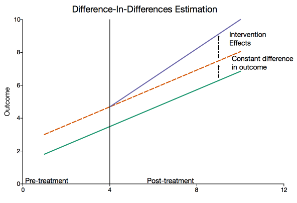
The dashed line continues the pre-treatment trend. The vertical gap is the effect.
3 point DiD. In the two-point approach we assume the same slope. With a third time point we also subtract the earlier gap in slopes, so a trend that already differed comes out of the effect, as long as that gap in slopes would have stayed constant.
DiD vs Matching. Difference-in-differences subtracts two changes. Matching only chooses who enters that subtraction.
Without matching, we choose the control group from domain knowledge: which group would have moved like the treated group if the intervention had not happened.