TL;DR
Kernel Density Estimation (KDE) is a statistical technique with applications across various fields, such as estimating the distribution of a random variable and computing the attention layer in Transformers. While the standard algorithm for KDE has a quadratic time complexity, this presentation introduces two advanced techniques (the polynomial method and the Fast Multipole Method) that reduce the computation time to nearly linear in certain cases.
KDE problem formulation
Inputs.
- \(2n\) points: \(x_1,x_2,...,x_n\) and \(y_1,y_2,...,y_n\). Each point is \(m\) dimensional.
- A weight vector \(w\) which is \(n\) dimensional.
- An error parameter \(\epsilon\).
- The kernel function \(f(x,y)\). \(K[i,j]=f(x_i,y_j)\)
The goal. Approximately compute (compute up an error) the multiplication \(Kw\)

A Naive algorithm is with a complexity of \(O(mn^2)\) with the following implementation:
- Constructing the matrix \(K\): Figuring out the \(m \times n\) entries of \(K\). Each \(f(x_i,j_i)\) is with \(m\) multiplications and there are \(n^2\) combinations the need to be evaluated.
- Multiple \(K\) by the vector \(w\). This adds additional \(n^2\) computations.
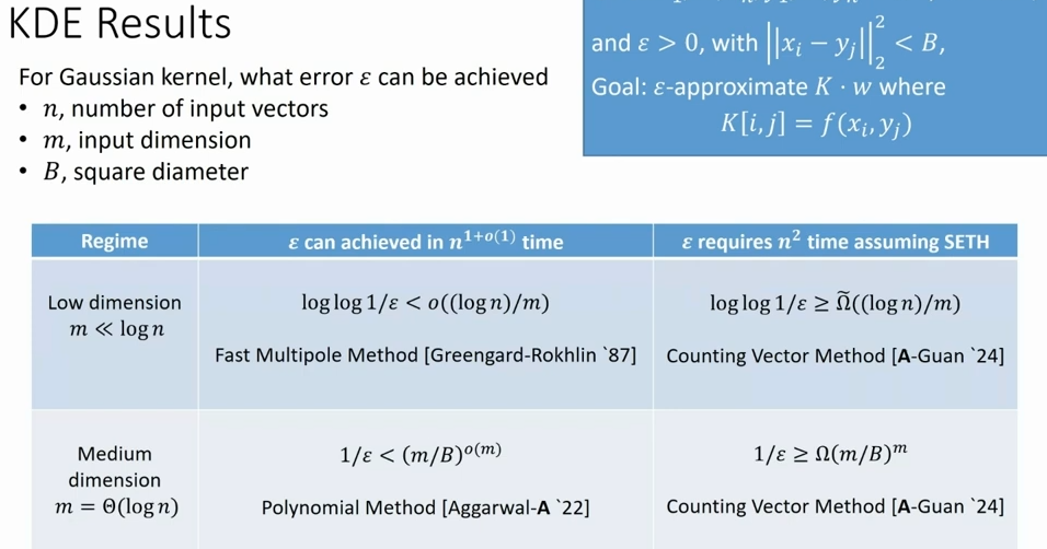
The KDE solution that is almost linear can be achieved based on the input dimension regime:
- Moderate dimension algorithm: The Polynomial method.
- Low dimensional algorithm: The Fast Multiple method.
KDE in practice
The most widespread kernel is the Gaussian Kernel:
$$f(x,y) = e^{||x-y||_2^2} $$KDE applications define different parameters regimes.
- Estimate the probability density function of a random variable: \(m << n\).
- n-body problem in physics: \(m << n\).
- Attention computation in Large Language Models: The attention matrix is a rescaling of the Gaussian Kernel matrix where \(n\) is the length of the context sequence and \(m\) is the vector size associate with a token. In the common case \(m = O(\log n)\).
Moderate dimension algorithm: The Polynomial method
- Find a low rank approximation for \(K\): \(LR^T=~K\)
- Compute \(Kw\) quickly with \(L(R^T w)\). This can be achieved by a polynomial approximation of \(e^{-x}\)
Chebyshev polynomials are a good approximators of e^{-x}
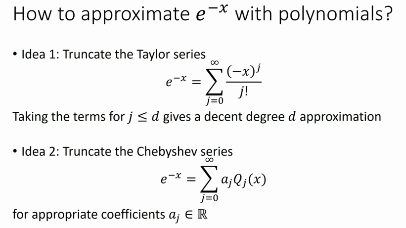 Using Chebyshev, less expansion terms (less \(j\)) are needed to reach a certain error bound compared to Taylor series.
Low dimensional algorithm: The Fast Multiple method
We can apply the same method of the Moderate dimension such that when \(m=O(1)\) we can get \(\epsilon = 1/poly(n)\). However, applying the Fast Multiple Method results is a better computational cost.
Steps:
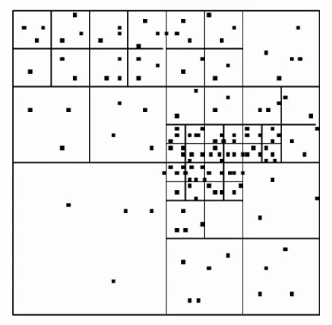
- Partition the space into boxes.
- Sum the contribution to \(Kw\) over pairs of nonempty boxes.
There can be \(n\) different boxes so we may up with \(n^2\) computations. We leverage the following insights.
- If boxes are far apart, their contribution to the summation is negligible and can be ignored.
- If boxes are well-separated, we can use constant degree polynomial.
- If boxes are too close, we keep partition the space to smaller boxes until one of the previous points are met.
Lower bound of KDE computation cost
The above algorithms are optimal: there’s a tight lower bound that shows we can not do better. The main idea of the lower bound proof is showing the problem of KDE is equivalent to solve the Hamming closest pair problem, which was already proven to require quadratic time.
Resource
Full results are summarized in this slide